Tutorial: Meshroom for Beginners
https://sketchfab.com/blogs/community/tutorial-meshroom-for-beginners
Goal
In this tutorial, we will explain how to use Meshroom to automatically create 3D models from a set of photographs. After specifying system requirements and installation, we will begin with some advice on image acquisition for photogrammetry. We will then give an overview of Meshroom UI and cover the basics by creating a project and starting the 3D reconstruction process. After that, we will see how the resulting mesh can be post-processed directly within Meshroom by applying an automatic decimation operation, and go on to learn how to retexture a modified mesh. We will sum up by showing how to use all this to work iteratively in Meshroom.
Finally, we will give some tips about uploading your 3D models to Sketchfab and conclude with useful links for further information.
Step 0: System requirements and installation
Meshroom software releases are self-contained portable packages. They are uploaded on the project’s GitHub page. To use Meshroom on your computer, simply download the proper release for your OS (Windows and Linux are supported), extract the archive and launch Meshroom executable.
Regarding hardware, an Nvidia GPU is required (with Compute Capability of at least 2.0) for the dense high quality mesh generation. 32GB of RAM is recommended for the meshing, but you can adjust parameters if you don’t meet this requirement.
Meshroom is released in open source under the permissive MPLv2 license, see Meshroom COPYING for more information.
Step 1: Image acquisition
The shooting quality is the most important and challenging part of the process. It has dramatic impacts on the quality of the final mesh.
The shooting is always a compromise to accomodate to the project’s goals and constraints: scene size, material properties, quality of the textures, shooting time, amount of light, varying light or objects, camera device’s quality and settings.
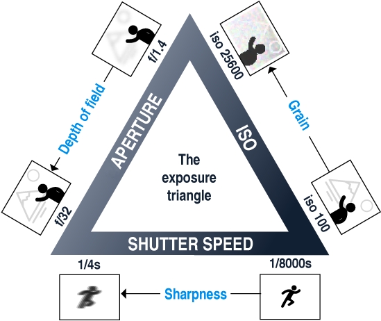
The main goal is to have sharp images without motion blur and without depth blur. So you should use tripods or fast shutter speed to avoid motion blur, reduce the aperture (high f-number) to have a large depth of field, and reduce the ISO to minimize the noise.
Step 2: Meshroom concept and UI overview
Meshroom has been conceived to address two main use-cases:
Easily obtain a 3D model from multiple images with minimal user action.
Provide advanced users (eg: expert graphic artists, researchers) with a solution that can be modified to suit their creative and/or technical needs.
For this reason, Meshroom relies on a nodal system which exposes all the photogrammetry pipeline steps as nodes with parameters. The high-level interface above this allows anyone to use Meshroom without the need to modify anything.
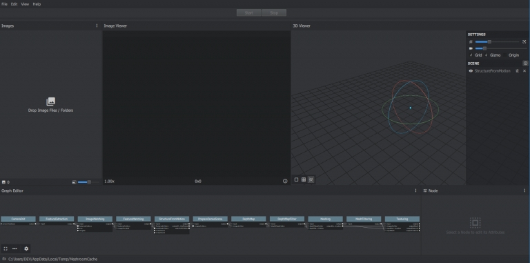
Meshroom User Interface
Step 3: Basic Workflow
For this first step, we will only use the high-level UI. Let’s save this
new project on our disk using “File  Save As…”.
All data computed by Meshroom will end up in a “MeshroomCache” folder next to this project file. Note that projects are portable: you can move the “.mg” file and its “MeshroomCache” folder afterwards. The cache location is indicated in the status bar, at the bottom of the window.
Next, we import images into this project by simply dropping them in the “Images” area – on the left-hand side. Meshroom analyzes their metadata and sets up the scene.
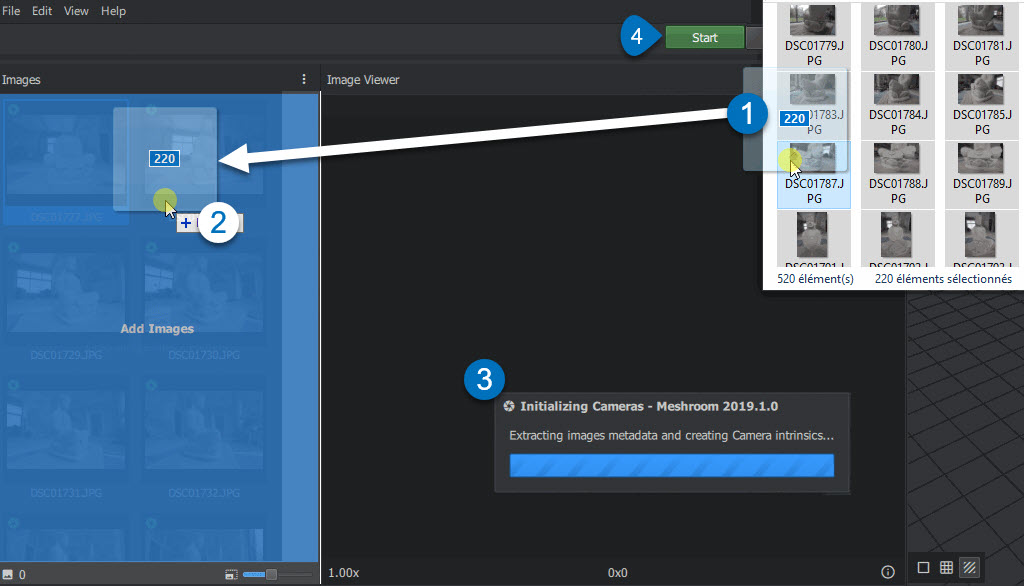
Meshroom relies on a Camera Sensors Database to determine camera internal parameters and group them together. If your images are missing metadata and/or were taken with a device unknown to Meshroom, an explicit warning will be displayed explaining the issue. In all cases, the process will go on but results might be degraded.
Once this is done, we can press the “Start” button and wait for the computation to finish. The colored progress bar helps follow the progress of each step in the process:
green: has been computed
orange: is being computed
blue: is submitted for computation
red: is in error
Step 4: Visualize and Export the results
The generic photogrammetry pipeline can be seen as having two main steps:
SfM: Structure-from-Motion (sparse reconstruction)
Infers the rigid scene structure (3D points) with the pose (position and orientation) and internal calibration of all cameras.
The result is a set of calibrated cameras with a sparse point cloud (in Alembic file format).
MVS: MultiView-Stereo (dense reconstruction)
Uses the calibrated cameras from the Structure-from-Motion to generate a dense geometric surface.
The final result is a textured mesh (in OBJ file format with the corresponding MTL and texture files).
As soon as the result of the “Structure-from-Motion” is available, it is automatically loaded by Meshroom. At this point, we can see which cameras have been successfully reconstructed in the “Images” panel (with a green camera icon) and visualize the 3D structure of the scene. We can also pick an image in the “Images” panel to see the corresponding camera in the 3D Viewer and vice-versa.
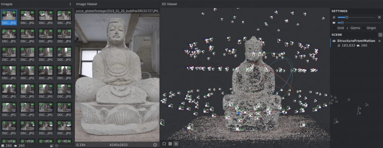
Image selection is synchronized between “Images” and “3D Viewer” panels.
3D Viewer interactions are mostly similar to Sketchfab’s:
Click and Move to rotate around view center
Double Click
on geometry (point cloud or mesh) to define view center
alternative: Ctrl+Click
Middle-Mouse Click
to pan
alternative: Shift+Click
Wheel Up/Down
to Zoom in/out
alternative: Alt+Right-Click and Move Left/Right
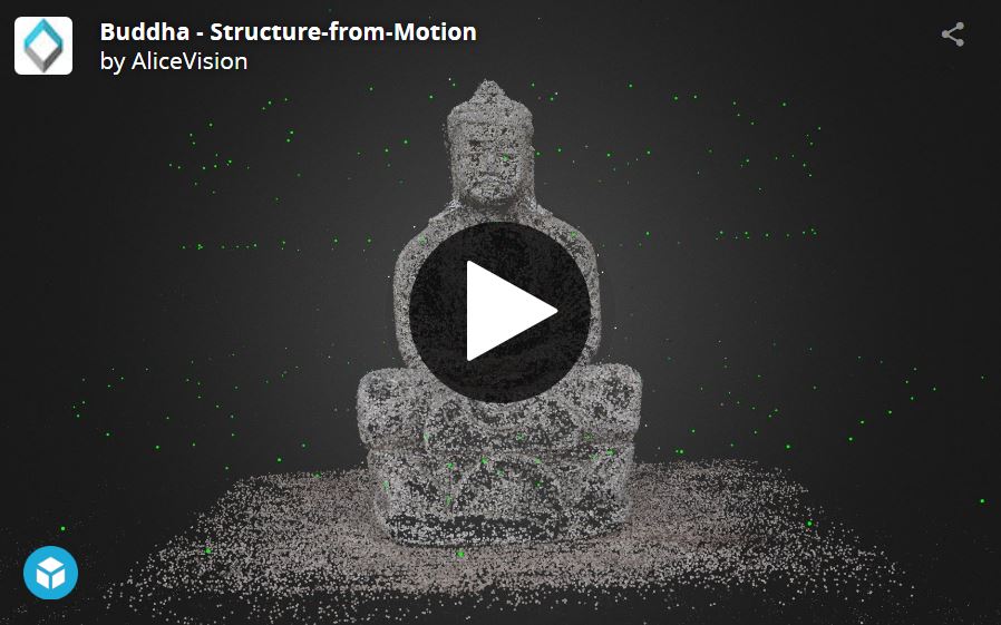
Buddha – Structure-from-Motion by AliceVision on Sketchfab
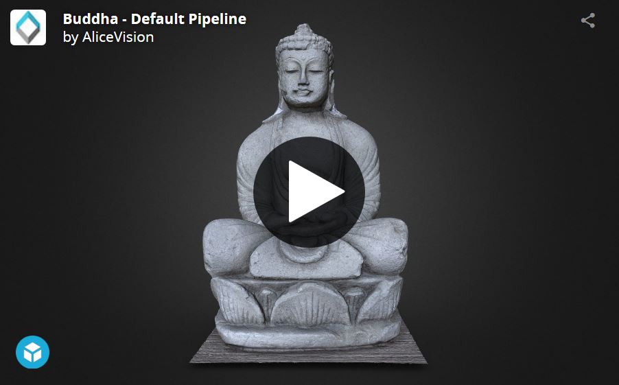
Once the whole pipeline has been computed, a “Load Model” button at the bottom of the 3D Viewer enables you to load and visualize the textured 3D mesh.
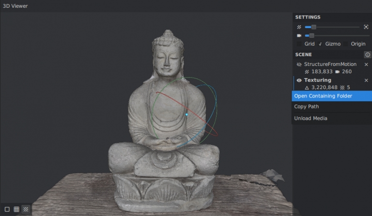
Visualize and access media files on disk from the 3D Viewer
There is no export step at the end of the process: the resulting files are already available on disk. You can right-click on a media and select “Open Containing Folder” to retrieve them. By doing so on “Texturing”, we get access to the folder containing the OBJ and texture files.
Step 5: Post-processing: Mesh Simplification
Let’s now see how the nodal system can be used to add a new process to this default pipeline. The goal of this step will be to create a low-poly version of our model using automatic mesh decimation.
Let’s move to the “Graph Editor” and right click in the empty space to open the node creation menu. From there, we select “MeshDecimate”: this creates a new node in the graph. Now, we need to give it the high-poly mesh as input. Let’s create a connection by clicking and dragging from MeshFiltering.output to MeshDecimate.input. We can now select the MeshDecimate node and adjust parameters to fit our needs, for example, by setting a maximum vertex count to 100,000. To start the computation, either press the main “Start” button, or right-click on a specific node and select “Compute”.
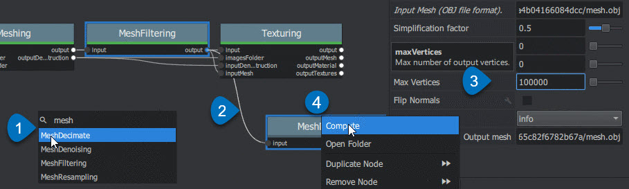
Create a MeshDecimate node, connect it, adjust parameters and start computation
By default, the graph will become read-only as soon as a computation is started in order to avoid any modification that would compromise the planned processes.
Each node that produces 3D media (point cloud or mesh) can be visualized in the 3D viewer by simply double-clicking on it. Let’s do that once the MeshDecimate node has been computed.
Double-Click on a node to visualize it in the 3D viewer. If the result is not yet computed, it will automatically be loaded once it’s available.
Ctrl+Click the visibility toggle of a media to display only this media alternative from Graph Editor: Ctrl+DoubleClick on a node
Step 6: Retexturing after Retopology
Making a variation of the original, high-poly mesh is only the first step to creating a tailored 3D model. Now, let’s see how we can re-texture this geometry.
Let’s head back to the Graph Editor and do the following operations:
Right Click on the Texturing node
DuplicateRight Click on the connection MeshFiltering.output
Texturing2.inputMesh RemoveCreate a connection from MeshDecimate.output to Texturing2.inputMesh
By doing so, we set up a texturing process that will use the result of the decimation as input geometry. We can now adjust the Texturing parameters if needed, and start the computation.
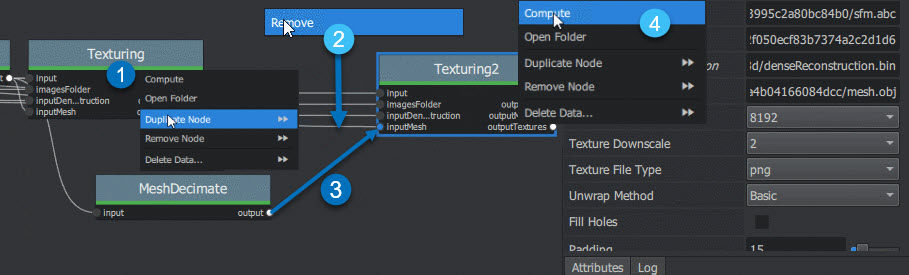
Retexture the decimated mesh using a second Texturing node
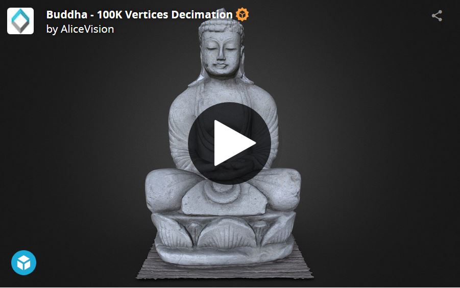
Buddha – 100K Vertices Decimation by AliceVision on Sketchfab
External retopology and custom UVs This setup can also be used to reproject textures on a mesh that has been modified outside Meshroom (e.g: retopology / unwrap). The only constraint is to stay in the same 3D space as the original reconstruction and therefore not change the scale or orientation.
Then, instead of connecting it to MeshDecimate.output, we would directly write the filepath of our mesh in Texturing2.inputMesh parameter from the node Attribute Editor. If this mesh already has UV coordinates, they will be used. Otherwise it will generate new UVs based on the chosen “Unwrap Method”.
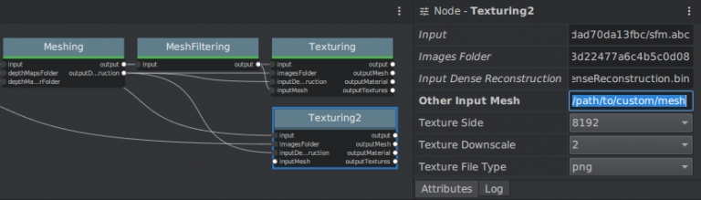
Texturing also accepts path to external meshes
Step 7: Draft Meshing from SfM
The MVS consists of creating depth maps for each camera, merging them together and using this huge amount of information to create a surface. The generation of those depth maps is, at the moment, the most computation intensive part of the pipeline and requires a CUDA enabled GPU. We will now explain how to generate a quick and rough mesh directly from the SfM output, in order to get a fast preview of the 3D model. To do that we will use the nodal system once again.
Let’s go back to the default pipeline and do the following operations:
Right Click
on DepthMap
Duplicate Nodes from Here
( “
” icon) to create a branch in the graph and keep the previous result available.
alternative: Alt + Click on the node
Select and remove (Right Click
Remove Node or Del)
DepthMap and DepthMapFilterConnect PrepareDenseScene.input
Meshing.inputConnect PrepareDenseScene.output
Texturing.inputImages
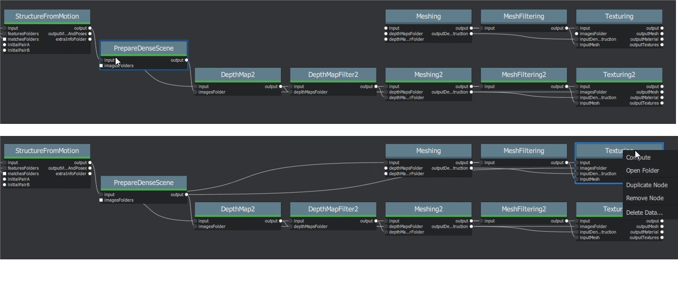
Draft Meshing from StructureFromMotion setup
With this shortcut, the Meshing directly uses the 3D points from the SfM, which bypass the computationally intensive steps and dramatically speed up the computation of the end of the pipeline. This also provides a solution to get a draft mesh without an Nvidia GPU.
The downside is that this technique will only work on highly textured datasets that can produce enough points in the sparse point cloud. In all cases, it won’t reach the level of quality and precision of the default pipeline, but it can be very useful to produce a preview during the acquisition or to get the 3D measurements before photo-modeling.
Step 8: Working Iteratively
We will now sum up by explaining how what we have learnt so far can be used to work iteratively and get the best results out of your datasets.
1. Computing and analyzing Structure-from-Motion first
This is the best way to check if the reconstruction is likely to be
successful before starting the rest of the process (Right click >
Compute on the StructureFromMotion node). The number of
reconstructed cameras and the aspect/density of the sparse point cloud
are good indicators for that. Several strategies can help improve
results at this early stage of the pipeline:
Extract more key points from input images by setting “Describer Preset” to “high” on FeatureExtraction node (or even “ultra” for small datasets).
Extract multiple types of key points by checking “akaze” in “Describer Type” on FeatureExtraction, FeatureMatching and StructureFromMotion nodes.
2. Using draft meshing from SfM to adjust parameters
Meshing the SfM output can also help to configure the parameters of the standard meshing process, by providing a fast preview of the dense reconstruction. Let’s look at this example:
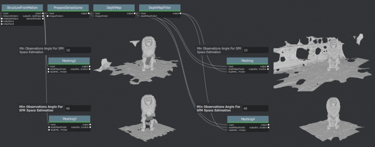
With the default parameters, we can preview from Meshing2 that the reconstructed area includes some parts of the environment that we don’t really want. By increasing the “Min Observations Angle For SfM Space Estimation” parameter, we are excluding points that are not supported by a strong angle constraint (Meshing3). This results in a narrower area without background elements at the end of the process (Meshing4 vs default Meshing).
\3. Experiment with parameters, create variants and compare results
One of the main advantages of the nodal system is the ability to create variations in the pipeline and compare them. Instead of changing a parameter on a node that has already been computed and invalidate it, we can duplicate it (or the whole branch), work on this copy and compare the variations to keep the best version.
In addition to what we have already covered in this tutorial, the most useful parameters to drive precision and performance for each step are detailed on the Meshroom Wiki.
Step 9: Upload results on Sketchfab
Results can be uploaded using the Sketchfab web interface, but Meshroom also provides an export tool to Sketchfab.
Our workflow mainly consists of these steps:
Decimate the mesh within Meshroom to reduce the number of polygons
Clean up this mesh in an external software, if required (to remove background elements for example)
Retexture the cleaned up mesh
Upload model and textures to Sketchfab
To directly publish your model from Meshroom, create a new SketchfabUpload node and connect it to the Texturing node.
You can see some 3D scans from the community here and on our Sketchfab page.
Don’t forget to tag your models with “alicevision” and “meshroom” if you want us to see your work!